Cars and Crime Symposium Workshop

Accessing and Analyzing UK Road Crash Data with stats19

Published

July 30, 2026

Welcome to the Cars and Crime Symposium Workshop repository!

Online Slides: robinlovelace.github.io/carscrime/slides.html
Source Code: github.com/Robinlovelace/carscrime

Last updated: July 30, 2026

Casualties over time

library(stats19)
library(tidyverse)
library(readr)

# Load pre-aggregated STATS19 dataset
cas_by_year_type <- read_csv("data/casualties_by_year_type.csv", show_col_types = FALSE)

# Absolute casualties over time
ggplot(cas_by_year_type, aes(x = collision_year, y = n, color = type)) +
  geom_line(linewidth = 1.2) +
  geom_point(size = 1.8) +
  scale_color_brewer(palette = "Set1") +
  labs(
    x = "Year", y = "Number of casualties", color = "Casualty Type",
    title = "UK Road Casualties by Transport Mode (1979 - Present)"
  ) +
  theme_minimal()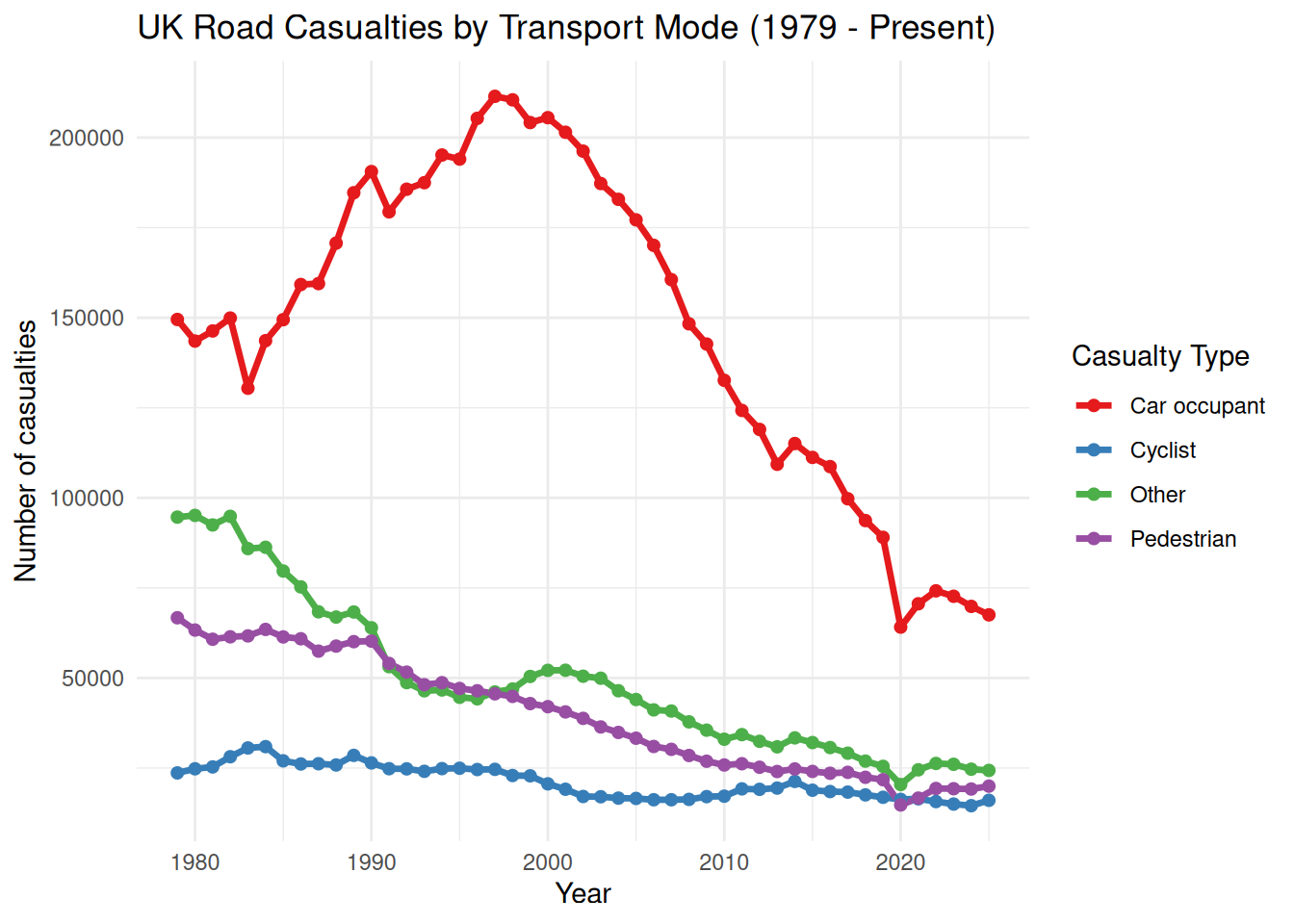

# Indexed plot (1979 = 100)
cas_1979 <- cas_by_year_type |>
  filter(collision_year == 1979) |>
  select(type, n) |>
  rename(n_1979 = n)

cas_by_year_type |>
  left_join(cas_1979, by = "type") |>
  mutate(n_indexed = n / n_1979 * 100) |>
  ggplot(aes(x = collision_year, y = n_indexed, color = type)) +
  geom_line(linewidth = 1.2) +
  scale_color_brewer(palette = "Set1") +
  labs(
    x = "Year", y = "Casualties indexed (1979 = 100)", color = "Casualty Type",
    title = "Relative Change in Casualties Since 1979"
  ) +
  theme_minimal()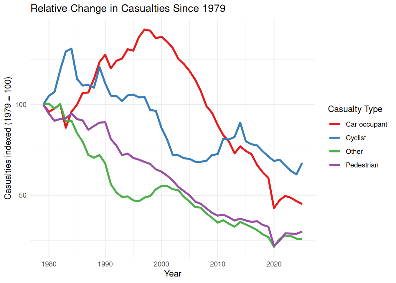

Car harms: How has the burden shifted?

The plots below illustrate how “car harms” have evolved differently for people driving, walking, and cycling.

Car occupant casualties — safety technology at work

Car occupant casualties have fallen dramatically since 1979, driven by seatbelt laws, airbags, crumple zones, and improved vehicle crash protection.

cas_by_year_type |>
  filter(type == "Car occupant") |>
  ggplot(aes(x = collision_year, y = n)) +
  geom_line(color = "#1F78B4", linewidth = 1.2) +
  geom_point(color = "#1F78B4", size = 2) +
  labs(
    x = "Year", y = "Car occupant casualties",
    subtitle = "Dramatic decline as vehicle safety improves for occupants inside cars"
  ) +
  theme_minimal()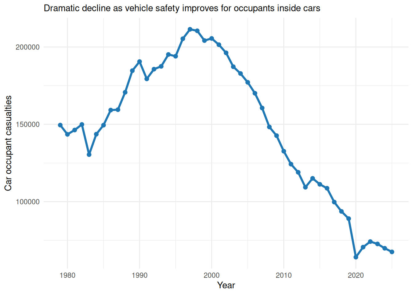

Pedestrians and Cyclists hit by cars: Hurt and Killed since 1979

By joining casualty data with vehicle table records, we isolate vulnerable road users (pedestrians and cyclists) struck in collisions involving cars, tracking how many were killed versus hurt (injured) each year since 1979.

vru_car_harm <- read_csv("data/vru_car_harm.csv", show_col_types = FALSE)

ggplot(vru_car_harm, aes(x = collision_year, y = n, color = outcome)) +
  geom_line(linewidth = 1.2) +
  facet_wrap(~ vru_mode, scales = "free_y") +
  scale_color_manual(values = c("Killed" = "#D95F02", "Hurt (Injured)" = "#7570B3")) +
  labs(
    x = "Year", y = "Number of casualties",
    title = "Pedestrians and Cyclists Hit by Cars (1979 - Present)",
    subtitle = "Annual counts of vulnerable road users killed vs hurt in car collisions",
    color = "Outcome"
  ) +
  theme_minimal()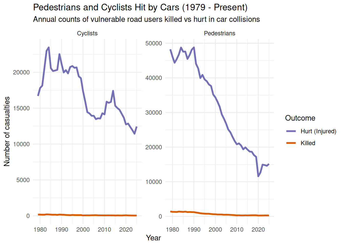

Risk shift: vulnerable road user casualties per car occupant

This ratio shows for every car occupant casualty, how many pedestrians and cyclists are hurt. A rising ratio indicates that the burden of risk has shifted onto people outside cars.

ratio_data <- cas_by_year_type |>
  filter(type %in% c("Car occupant", "Pedestrian", "Cyclist")) |>
  pivot_wider(names_from = type, values_from = n) |>
  mutate(
    ped_per_car = Pedestrian / `Car occupant`,
    cycle_per_car = Cyclist / `Car occupant`
  )

ggplot(ratio_data, aes(x = collision_year)) +
  geom_line(aes(y = ped_per_car, color = "Pedestrians per car occupant"), linewidth = 1.2) +
  geom_point(aes(y = ped_per_car, color = "Pedestrians per car occupant"), size = 1.8) +
  geom_line(aes(y = cycle_per_car, color = "Cyclists per car occupant"), linewidth = 1.2) +
  geom_point(aes(y = cycle_per_car, color = "Cyclists per car occupant"), size = 1.8) +
  scale_color_manual(values = c("Pedestrians per car occupant" = "#E7298A",
                                 "Cyclists per car occupant" = "#66A61E")) +
  labs(
    x = "Year", y = "Casualty ratio",
    color = NULL,
    subtitle = "Risk burden has shifted from car occupants to vulnerable road users"
  ) +
  theme_minimal()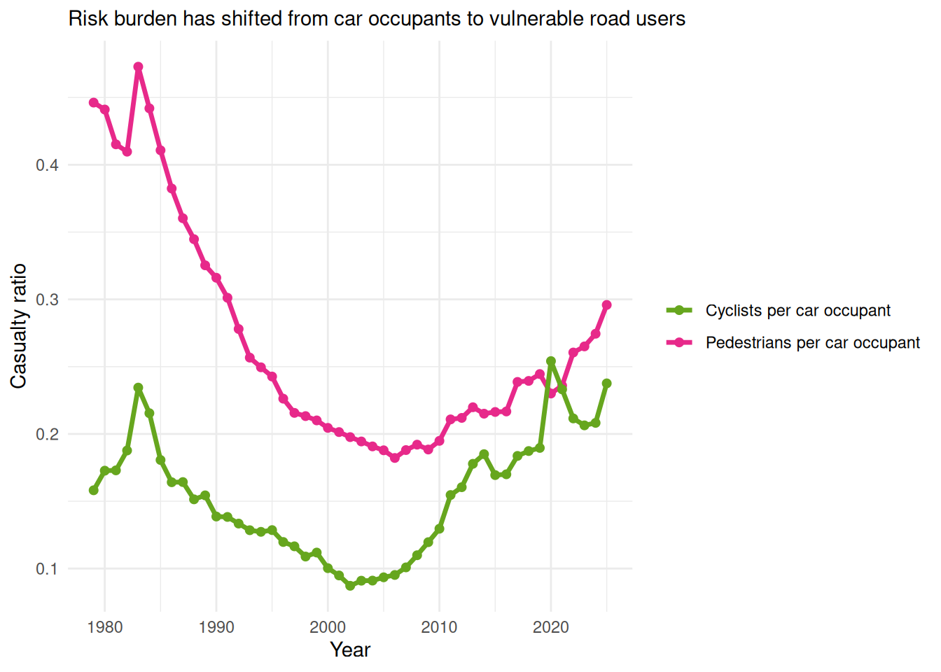

Additional Trends in Car Harms

Trend 1: Car size & engine capacity inflation (`engine_capacity_cc`) over time

As cars have grown heavier, wider, and more powerful (the “SUV-ification” of passenger vehicles), average engine displacement of cars involved in collisions with pedestrians and cyclists has steadily increased.

car_engine_vru <- read_csv("data/car_engine_vru.csv", show_col_types = FALSE)

ggplot(car_engine_vru, aes(x = collision_year)) +
  geom_line(aes(y = mean_cc, color = "Mean engine capacity (cc)"), linewidth = 1.2) +
  geom_line(aes(y = median_cc, color = "Median engine capacity (cc)"), linewidth = 1.2, linetype = "dashed") +
  scale_color_manual(values = c("Mean engine capacity (cc)" = "#D95F02",
                                 "Median engine capacity (cc)" = "#1B9E77")) +
  labs(
    x = "Year", y = "Engine capacity (cc)",
    color = "Metric",
    title = "Engine Capacity of Cars Involved in Vulnerable Road User Collisions",
    subtitle = "Steady rise in engine size of cars striking pedestrians and cyclists"
  ) +
  theme_minimal()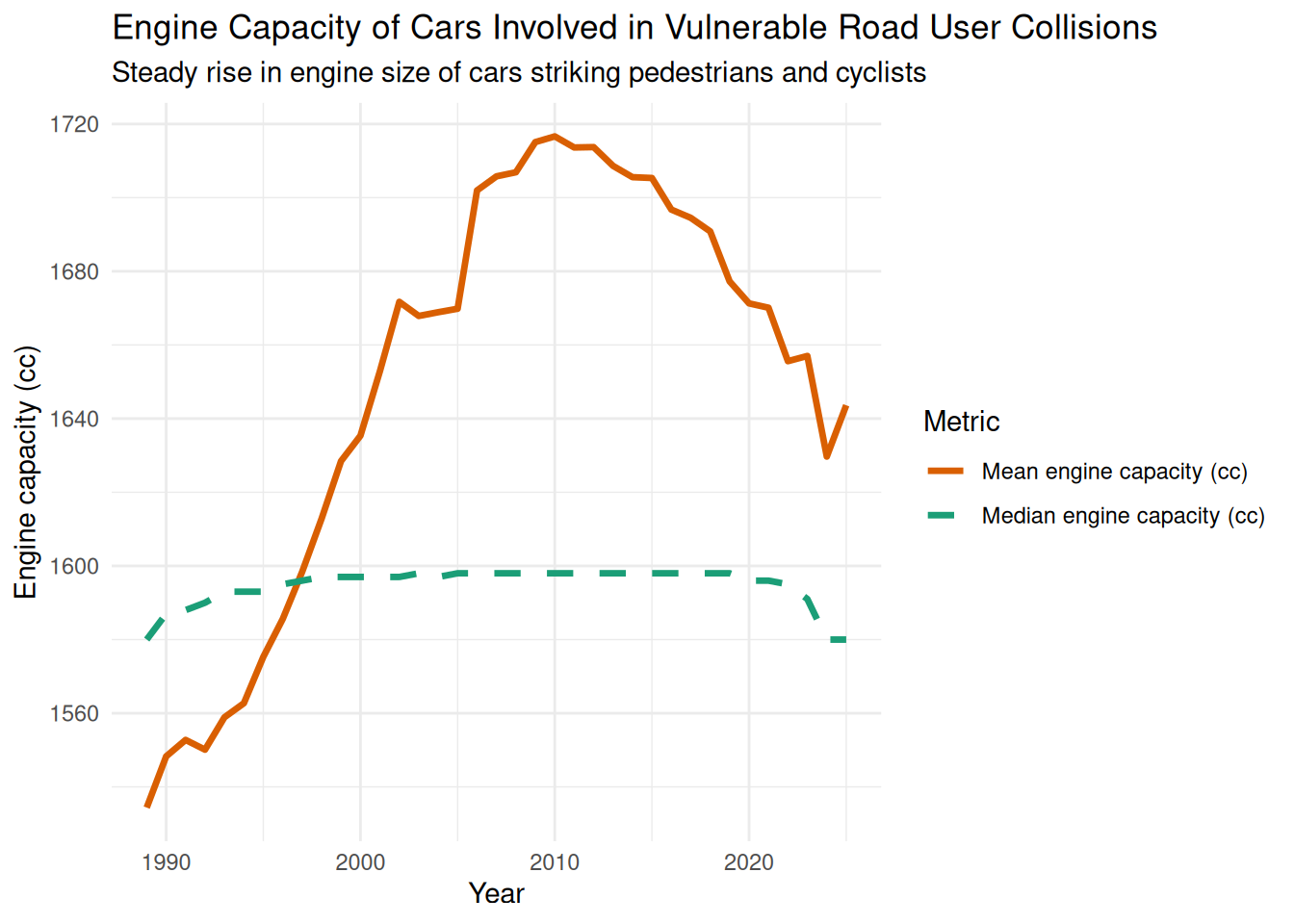

Trend 2: Driver Sex in Vulnerable Road User Collisions

Analyzing vehicle driver attributes shows a persistent, large disparity in driver sex for cars involved in collisions striking pedestrians and cyclists.

driver_sex_vru <- read_csv("data/driver_sex_vru.csv", show_col_types = FALSE)

ggplot(driver_sex_vru, aes(x = collision_year, y = n, color = sex_of_driver)) +
  geom_line(linewidth = 1.2) +
  scale_color_manual(values = c("Male" = "#377EB8", "Female" = "#E41A1C")) +
  labs(
    x = "Year", y = "Number of drivers in VRU collisions",
    color = "Driver Sex",
    title = "Driver Sex in Car Collisions Involving Pedestrians and Cyclists",
    subtitle = "Male drivers account for the majority of cars involved in VRU collisions"
  ) +
  theme_minimal()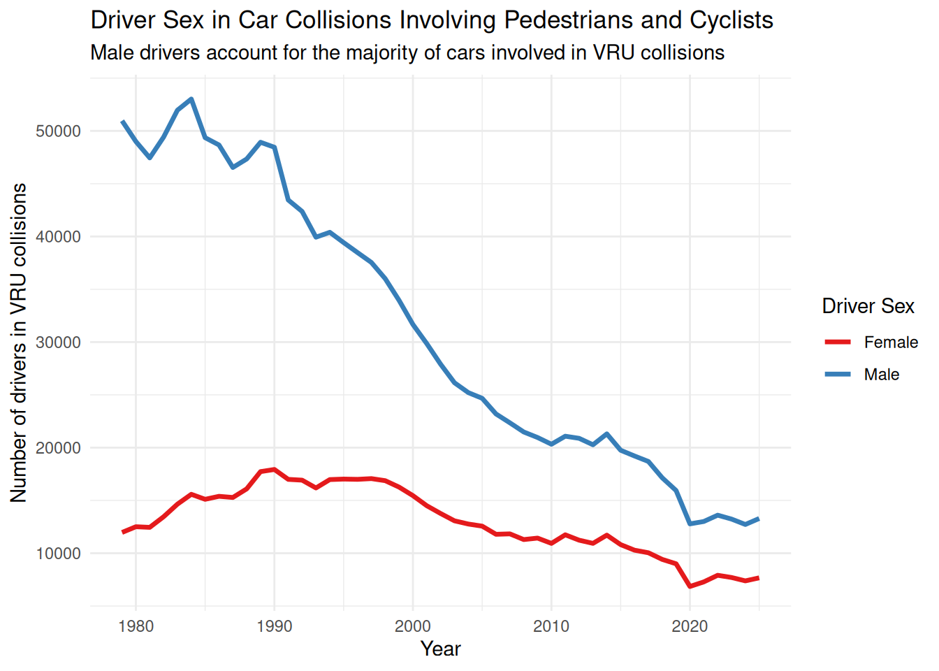

Overview

This repository contains reproducible slides and materials for the Cars and Crime Symposium Workshop on accessing and analyzing UK road safety data using the {stats19} R package.

Workshop Agenda (60 Mins)

00:00 – 00:15: Introduction to STATS19 & {stats19} R package (3 core tables architecture).
00:15 – 00:30: Research Topics & Methodological Challenges (TBC).
00:30 – 01:00: Breakout Workshop Groups:
- Group 1 (Robin): Hands-on code & vignette walkthrough.
- Group 2 (Roger): Research design & analysis plans.
- Group 3: Informal walk & networking.

Getting Started

You can launch an interactive R development environment directly in your browser:

Open in GitHub Codespaces